Estimate distribution from sample

Problem Create a pdqr-function representing an estimation of sample’s distribution.

Solution The most important decision here is about distribution’s type: discrete or continuous. In first case, any new_*() function will use unique values of sample as distribution’s outcomes, and probabilities will be estimated by tabulating and normalizing:

# Any pdqr class can be used to represent distribution
mpg_dis <- new_d(mtcars$mpg, type = "discrete")

# Pdqr-functions have `print()` methods with concise summary
mpg_dis
## Probability mass function of discrete type
## Support: [10.4, 33.9] (25 elements)

# To visually inspect pdqr-function, use `plot()`
plot(mpg_dis)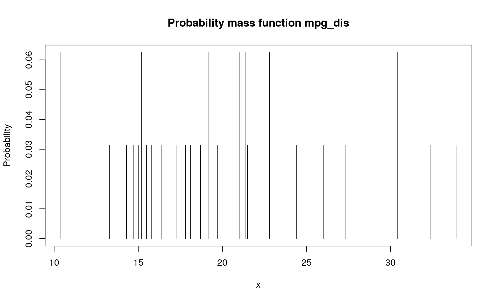

For continuous type, density() function will be used to estimate distribution’s density (if sample has 2 or more elements). Note that arguments of density() will affect greatly the output distribution (as always with kernel density estimation).

mpg_con <- new_d(mtcars$mpg, type = "continuous")
mpg_con
## Density function of continuous type
## Support: ~[2.96996, 41.33004] (511 intervals)

plot(mpg_con)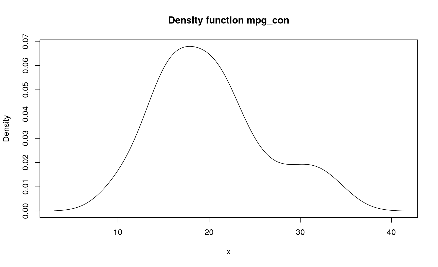

These newly created functions can be used to obtain probability or density of any point:

# Probabilities
mpg_dis(20:25)
## [1] 0.0000 0.0625 0.0000 0.0000 0.0000 0.0000

# Density values
mpg_con(20:25)
## [1] 0.06469730 0.06040205 0.05394401 0.04591992 0.03759639 0.03029240

Estimate distribution of positive values

Problem Create a pdqr-function representing an estimation of sample’s distribution with assumption that it can produce only positive values.

Solution This common task is done in two steps:

• Estimate sample distribution, as in previous step. It can result into unwanted distribution properties, like producing negative values. This is a known issue of boundary problem in kernel density estimation.
• Modify distribution to have only positive support with form_resupport(). It has several methods with default one ("reflect") recommended to deal with boundary correction. It “reflects” density tails “inside” of a desired support interval. Its output for bounded distributions is usually a closer estimation of “true distribution”.

# Exponential distribution can have only positive values
exp_sample <- rexp(100)
d_exp <- new_d(exp_sample, type = "continuous")

  # Use `NA` to indicate that certain edge of support should remain unchanged
d_exp_corr <- form_resupport(d_exp, support = c(0, NA))
  # Original kernel density estimation
plot(
  d_exp, main = "Different estimations of exponential distribution",
  ylim = c(0, 1)
)
  # Corrected density
lines(d_exp_corr, col = "blue")
  # Reference distribution
lines(seq(0, 6, by = 0.01), dexp(seq(0, 6, by = 0.01)), col = "red")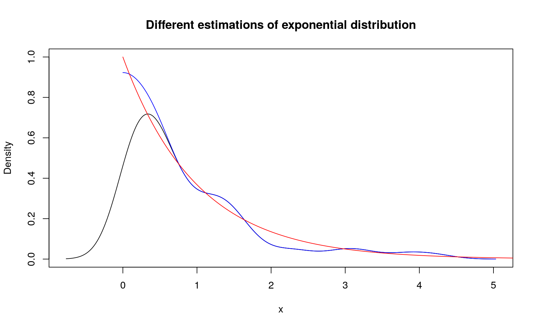

Generate sample similar to input

Problem Generate sample of certain size from distribution that is an estimate to original sample’s distribution.

Solution R-functions are used for generating samples. There are two ways of creating them:

# Create new r-function from sample
r_mpg_dis <- new_r(mtcars$mpg, type = "discrete")
r_mpg_dis(n = 10)
##  [1] 15.2 15.2 10.4 16.4 15.5 30.4 18.1 21.5 30.4 15.2

# Convert existing pdqr-function to be r-function
r_mpg_con <- as_r(mpg_con)
r_mpg_con(n = 10)
##  [1] 18.68990 20.91834 20.22863 15.94346 15.12797 35.04418 12.48795
##  [8] 28.79146 15.24957 24.35035

Compute sum of random variables

Problem Compute pdqr-function representing sum of two independent random variables (for example, both being standard normal distributions).

Solution First, you need to create pdqr-functions for random variables. Here standard normal distribution will be used. This can be done by converting base R distribution functions to be pdqr-functions. After that, using + gives distribution of sum of two random variables:

(d_norm <- as_d(dnorm))
## Density function of continuous type
## Support: ~[-4.75342, 4.75342] (10000 intervals)
(d_norm_sum <- d_norm + d_norm)
## Density function of continuous type
## Support: ~[-5.69484, 6.37105] (511 intervals)

plot(d_norm_sum, main = "Sum of two standard normal distributions")
  # "True" sum of two independent normal random variables
lines(as_d(dnorm, sd = sqrt(2)), col = "red")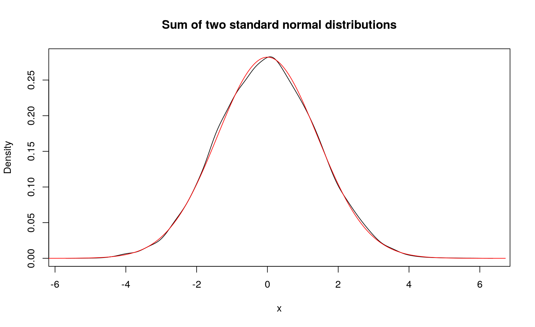

Here you can see two very important features of ‘pdqr’:

• Normal distribution is approximated with piecewise-linear density on finite support (10000 intervals are used by default).
• Distribution of sum of random variables is computed with simulation: large samples are drawn from both distributions, sums of their values are computed (resulting in a sample from sum of random variables), and target distribution is created using one of new_*() functions.

Compute mixture

Problem Compute mixture of distributions with different weights.

Solution Specifically for this task, there is a form_mix() function. It takes a list of pdqr-functions with, possibly, a vector of their weights in mixture:

d_norm_list <- list(as_d(dnorm), as_d(dnorm, mean = 3, sd = 0.7))
(d_norm_mix <- form_mix(d_norm_list, weights = c(0.2, 0.8)))
## Density function of continuous type
## Support: ~[-4.75342, 6.3274] (20003 intervals)

plot(d_norm_mix)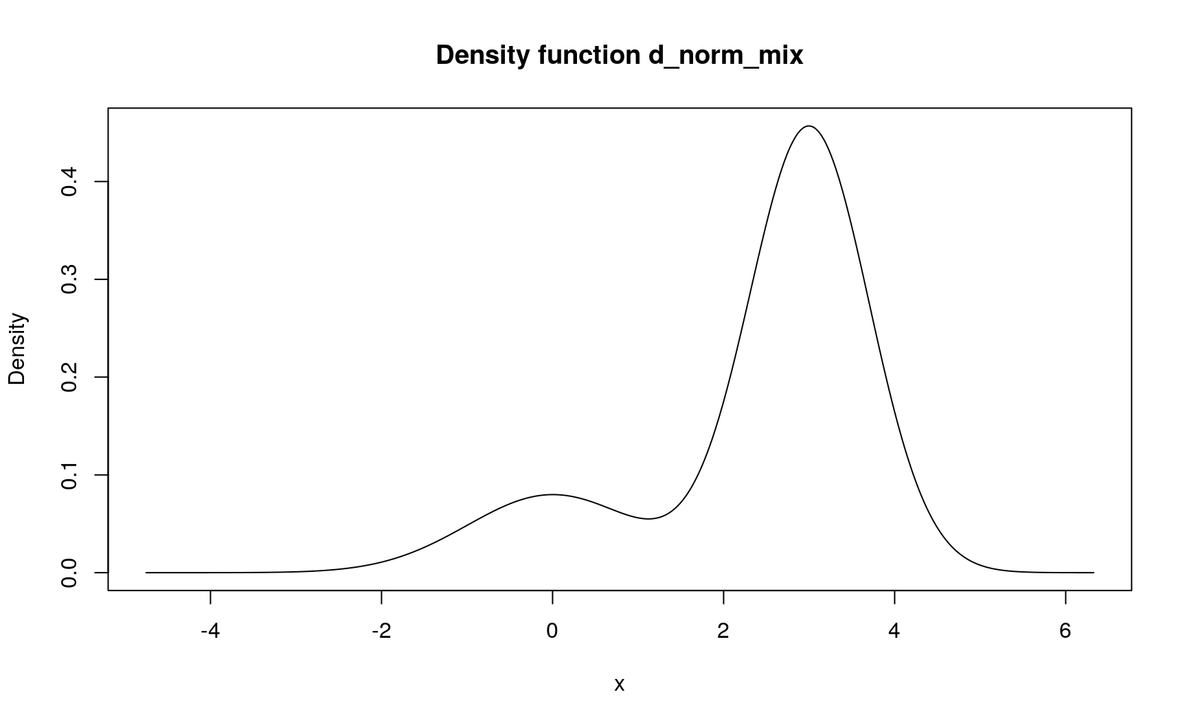

# As with other pdqr-functions, it can be used for obtaining values
d_norm_mix(seq(-1, 1, by = 0.2))
##  [1] 0.04839424 0.05793842 0.06664505 0.07365417 0.07822190 0.07983544
##  [7] 0.07836164 0.07411459 0.06792242 0.06120445 0.05609038

Compute winsorized sample mean

Problem Compute 10% winsorized sample mean.

Solution This can be done by purposefully separating task into three steps:

• Estimate sample distribution. It can have any type, depending on problem. Type “discrete” is better suited to emulate traditional sample estimates.
• Transform distribution by winsorizing tails. There is a form_tails() functions, which takes pdqr-function and returns pdqr-function for distribution with modified tails (based on supplied method).
• Compute mean of winsorized distribution. Note that in case of other statistic (like variance, skewness, etc.) no bias correction is done: output is a summary of distribution created on previous step(s).

mtcars$mpg %>% 
  new_d(type = "discrete") %>% 
  form_tails(level = 0.1, method = "winsor", direction = "both") %>% 
  summ_mean()
## [1] 20.19375

Compute mode

Problem Compute mode of distribution based on its sample.

Solution Use summ_mode():

mtcars$mpg %>% 
  # Using "continuous" type will smooth input to get mode of density curve.
  # With type "discrete" the most frequent input value is returned.
  new_d(type = "continuous") %>% 
  summ_mode()
## [1] 17.90862

Compute highest density region

Problem Compute 90% highest density region (HDR) of a distribution.

Solution There is a summ_hdr() function for this task. On a one dimensional line, HDR can only be a union of disjoint intervals. So the output of summ_hdr() is a region - data frame with rows representing different intervals of the union and two columns “left” and “right” for left and right ends of intervals.

norm_mix <- form_mix(
  list(as_d(dnorm), as_d(dnorm, mean = 5)),
  weights = c(0.3, 0.7)
)
(norm_mix_hdr <- summ_hdr(norm_mix, level = 0.9))
##        left    right
## 1 -1.342624 1.348071
## 2  3.119697 6.870090

There is a region_*() family of functions to work with regions. Here are several examples:

# Test if number is inside region
region_is_in(norm_mix_hdr, x = c(-10, 0, 3, 10))
## [1] FALSE  TRUE FALSE FALSE

# Compute region width (sum of widths of all disjoint intervals)
region_width(norm_mix_hdr)
## [1] 6.441087

# Draw regions
plot(norm_mix)
region_draw(norm_mix_hdr)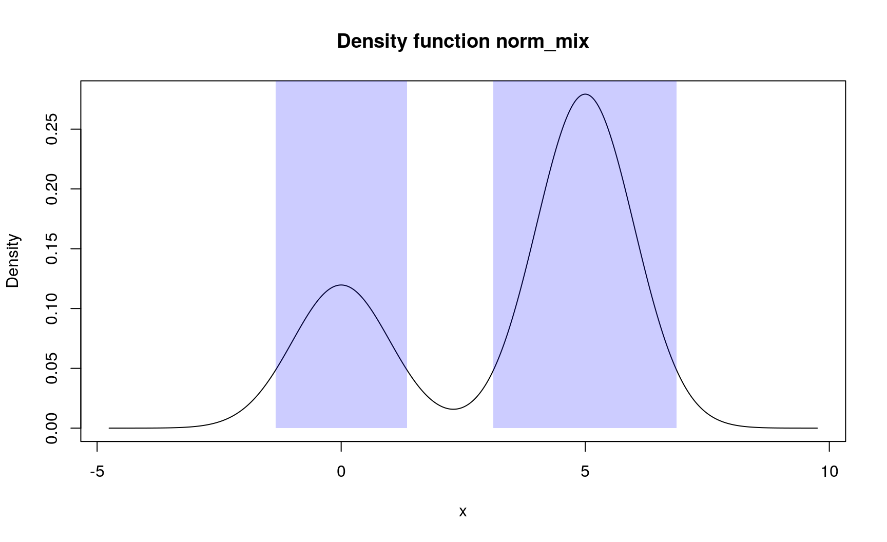

Compute separation threshold

Problem Compute a numerical threshold that optimally separates two distributions.

Solution There is a summ_separation() function designed specifically for this type of problem. It has several methods with default one being “KS” (short for “Kolmogorov-Smirnov”): optimal separation is done at point where two CDFs differ the most.

x <- rnorm(100)
y <- rnorm(100, mean = 2)
# Here "true optimal" is 1
summ_separation(f = new_d(x, "continuous"), g = new_d(y, "continuous"))
## [1] 0.9763479

Compute probability of being greater

Problem Compute a probability that random draw from one distribution is greater than random draw from another distribution.

Solution These type of summaries are usually done in two steps:

• Compute a boolean pdqr-function that represents a result of comparison between mentioned two random draws. It is a special kind of discrete distribution: it only has values 0 and 1 representing estimated relation being false and true respectively. Usually, they are the output of base R comparison operators: >, <, ==, etc.
• Extract a probability of a relation being true.

d_norm <- as_d(dnorm)
d_unif <- as_d(dunif)

# The output of `>` is a boolean pdqr-function. For convenience, printing
# displays also a probability of 1, which is a probability of relation being
# true. In this case, it should be read as "probability that random draw from
# first distribution is greater than a random draw from second one".
(norm_geq_unif <- d_norm > d_unif)
## Probability mass function of discrete type
## Support: [0, 1] (2 elements, probability of 1: ~0.31563)

# Extract desired probability
summ_prob_true(norm_geq_unif)
## [1] 0.3156265

Compute distance between distributions

Problem Compute distance between two distributions: positive value indicating “how far” two distributions are from each other. This is usually needed when comparing random outcomes of two (or more) options.

Solution There is a summ_distance() function with many methods.

# Default method is "KS" (short for "Kolmogorov-Smirnov"): the biggest
# absolute difference between two CDFs
summ_distance(d_norm, d_unif, method = "KS")
## [1] 0.5

# There is also "wass" method (short for "Wasserstein"): average path density
# point should go while transforming from one into another
summ_distance(d_norm, d_unif, method = "wass")
## [1] 0.7006094