Bandwidth bw

Argument bw is responsible for computing bandwith of kernel density estimation: one of the main parameters that greatly affect the output. It can be specified as either algorithm of computation or directly as number. Because actual bandwidth is computed as adjust*bw (adjust is another density() argument, which is explored in the next section), here we will see how different algorithms compute bandwidths, and the effect of changing numeric value of bandwidth will be shown in section about adjust.

There are 5 available algorithms: “nrd0”, “nrd”, “ucv”, “bcv”, “SJ”. Here is an animation of their effect:

density_anim(bw = c("nrd0", "nrd", "ucv", "bcv", "SJ"), duration = 5)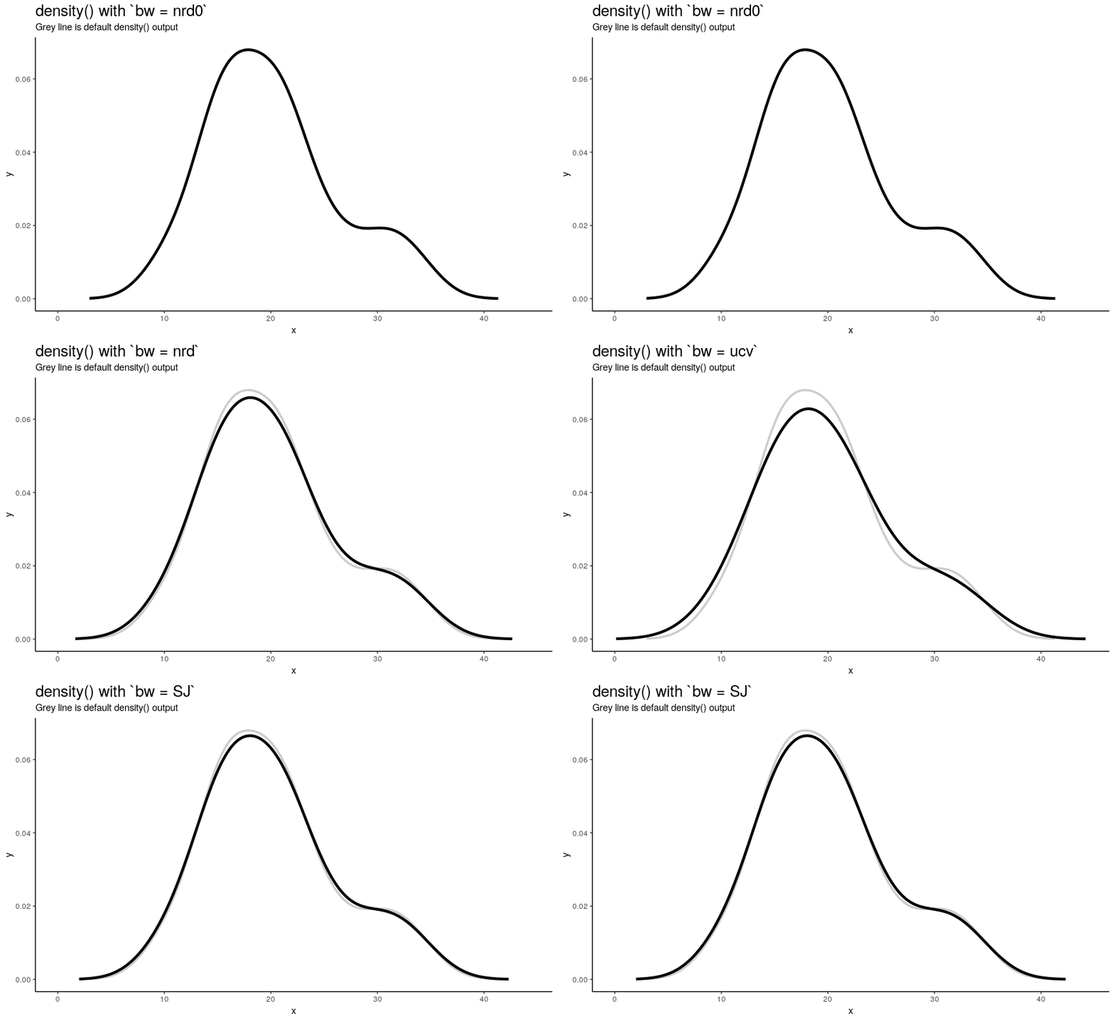

As you can see, density curve changes, but not drastically. At least the whole shape seems to be somewhat preserved.

Adjusting bandwidth adjust

To easily “specify values like ‘half the default’ bandwidth”, there is an argument adjust. Bigger values indicate greater bandwidth that is actually used. Zero results into zero bandwidth (so never should be used), one (default) - into originally computed by chosen algorithm.

density_anim(adjust = seq(0.1, 2, by = 0.05))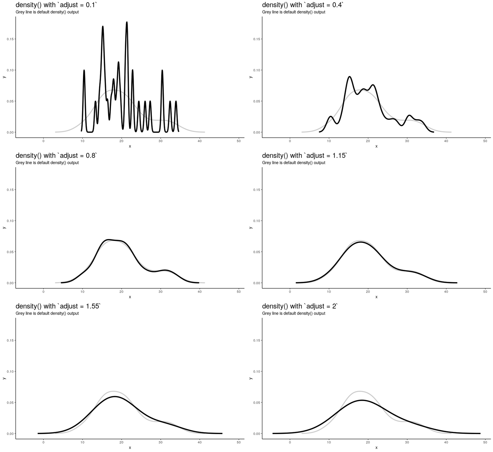

Changing adjust leads to very noticeable changes in output shape of density curve: bigger values give smoother curves.

Kernel type kernel

Argument kernel defines the shape of kernel which will be used. There are 7 possible kernels in total which are shown in the following animation:

density_anim(
  kernel = c("gaussian", "epanechnikov", "rectangular", "triangular",
             "biweight", "cosine", "optcosine"),
  duration = 7
)

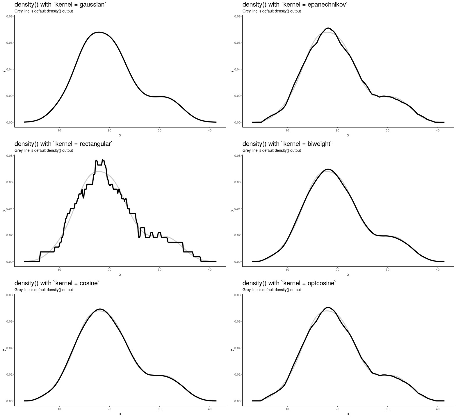
Choice of kernel function also considerably affects the output shape of density curve, but not as greatly as adjust. Most notable difference from default “gaussian” kernel is with “rectangular” kernel: result, unsurprisingly, is “more rectangular”.

Observation importance weights

Argument weights should be used if some observations are considered to be “more important” and are “more reference” than the other ones. It should be a numeric vector with the same length as input sample x. Note that for output to be a true density plot, sum of weights should be 1.

To illustrate its effect, lets construct a sequence of weights each of which makes one observation having 10 times more weight than any other (that contribute equally). Order of those observations we will choose so that they progress from the smallest to the biggest.

weights_list <- lapply(order(mtcars$mpg), function(i) {
  res <- c(rep(1, times = i-1), 10, rep(1, times = length(mtcars$mpg)-i))
  
  res / sum(res)
})

density_anim(weights = weights_list)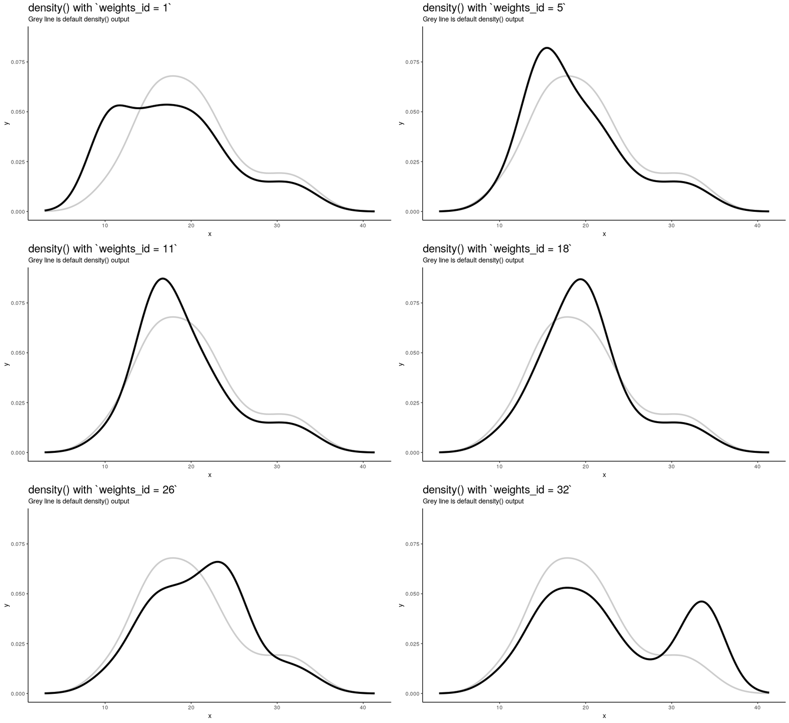

As expected from weights_list construction, one can see a “spike” that “travels” from left to right, indicating the position of “most important” observation.

Number of points n

n is responsible for number of returned x-y points. They are equally spaced on the specified range (see next sections). Default value is 512 (taken as a power of two for performance reasons of fft()), but to illustrate its effect on output lets use sequence from 2 to 50.

density_anim(n = 2:50)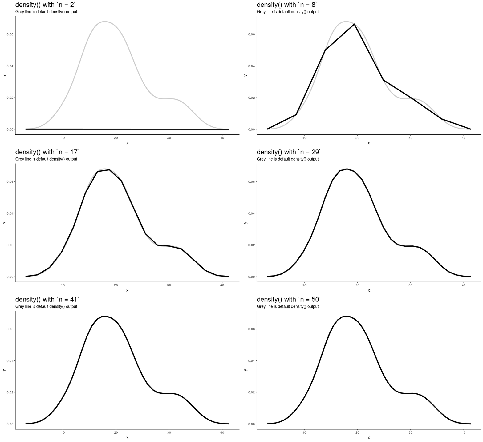

As you can see, in this case values higher than 40 already give considerably small errors (compared to “true curve” when n is infinity). However, if the underlying curve isn’t that smooth (for example, in case of low adjust) it is a good idea to use more points with default 512 being enough for most practical situations.

Left edge from

If specified, from defines a left edge of sequence of “x” points, at which density curve is evaluated. For illustration, lets use sequence from minimum to maximum values of mtcars$mpg.

from_vec <- seq(from = min(mtcars$mpg), to = max(mtcars$mpg), length.out = 20)

density_anim(from = round(from_vec, digits = 1))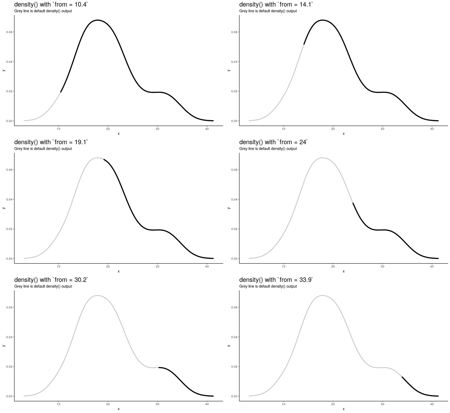

Note that when from is equal to the smallest value of input numeric vector, it is still greater than left edge of default density curve. For explanation of this “extending property” of default curve, see section about cut.

Right edge to

Argument to has the same nature as from, but defines right edge of points.

to_vec <- rev(from_vec)

density_anim(to = round(to_vec, digits = 1))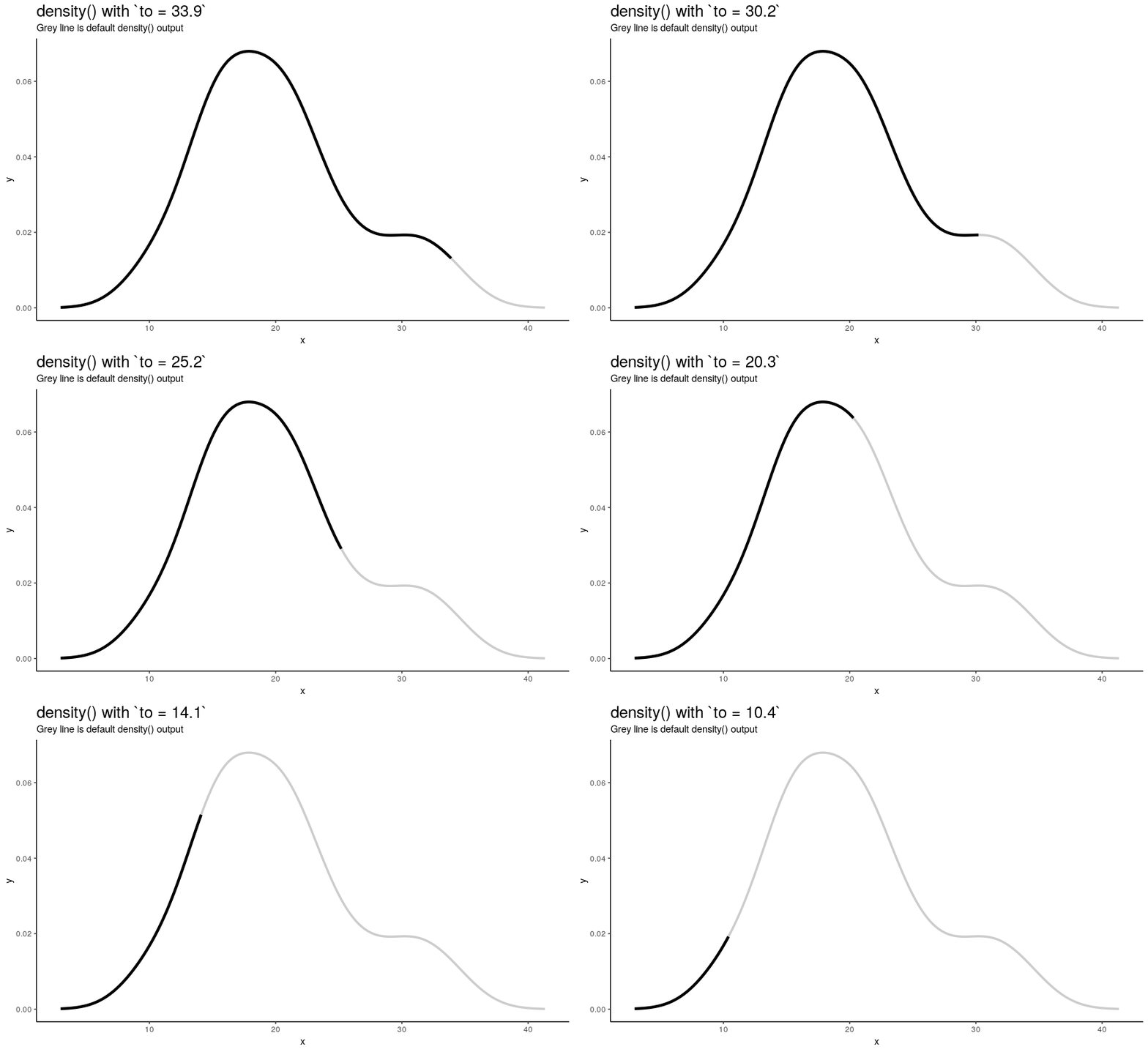

Note again, that value of to equal to maximum of input numeric vector is not enough to see the default behavior.

Range extension cut

By default, sequence of n x-y points is computed as follows:

• Equally spaced grid of n “x” points is computed between from and to which by default are computed as being “cut*bw outside of range(x)”. In other words, default range is extended to left and right of range(x) by the amount of “canonical bandwidth” (computed by bw algorithm) multiplied by argument cut (default being 3).
• “Y” points are taken from “true curve” of kernel density estimate.

density_anim(cut = seq(3, 0, by = -0.2))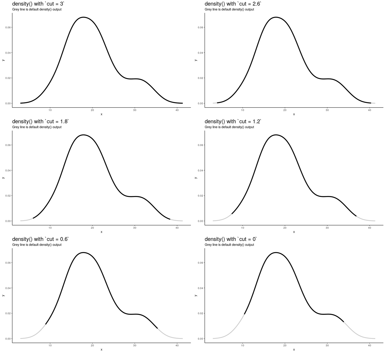

When cut changes from 3 to 0, range of computed points shrinks from default one to range of input numeric vector. Default call to density() computes set of points outside of original range. I call this behavior an “extending property” of density(). Note that cut can also be negative, which means reduced input range.

So by default, density() extends range of input vector. The problem is that it can contradict natural constraints on input. For example, what if you want to estimate density for probability distribution of value that can only be positive? Dealing with boundary values during kernel density estimation is an important topic and it is called a boundary correction problem. One of possible solutions is to use form_resupport() function from ‘pdqr’ package.