Example 1: single numerical estimate

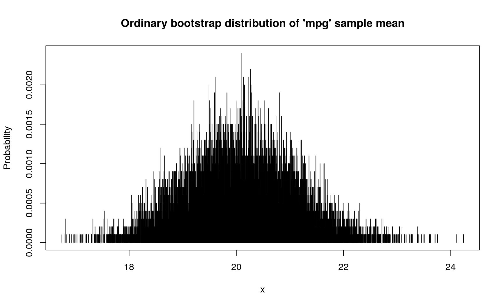
Mean value of ‘mpg’ variable in mtcars dataset is 20.090625. However, having in mind statistical uncertainty, we can ask how precise is this estimation? This can, and should, be reformulated in the following question: if we repeat sampling sets of 32 cars from general population of all cars, how close their ‘mpg’ sample means will be to each other? This can be answered by computing bootstrap distribution of sample means (pipe %>% function from ‘magrittr’ package is used to simplify notation):

# Using ordinary bootstrap
d_mpg_dis_mean <- mtcars$mpg %>% 
  new_d(type = "discrete") %>% 
  form_estimate(stat = mean, sample_size = nrow(mtcars))

  # Spread of this bootstrap distribution describes the precision of estimation:
  # bigger values indicate lower precision
summ_sd(d_mpg_dis_mean)
## [1] 1.04067

  # This discrete distribution has the following d-function
plot(
  d_mpg_dis_mean,
  main = "Ordinary bootstrap distribution of 'mpg' sample mean"
)

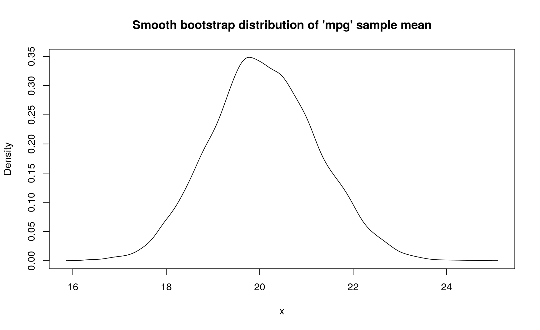
If modeling assumption about continuous nature of ‘mpg’ variable is reasonable (which it seems so), you can use “smooth bootstrap” by changing type of initial pdqr-function:

# Using smooth bootstrap with `type = "continuous"`
d_mpg_con_mean <- mtcars$mpg %>% 
  new_d(type = "continuous") %>% 
  form_estimate(stat = mean, sample_size = nrow(mtcars))

  # Spread is higher in this case because kernel density estimation with
  # `density()` function extends support during creation of pdqr-function on the
  # bootstrap step
summ_sd(d_mpg_con_mean)
## [1] 1.153957

plot(
  d_mpg_con_mean,
  main = "Smooth bootstrap distribution of 'mpg' sample mean"
)

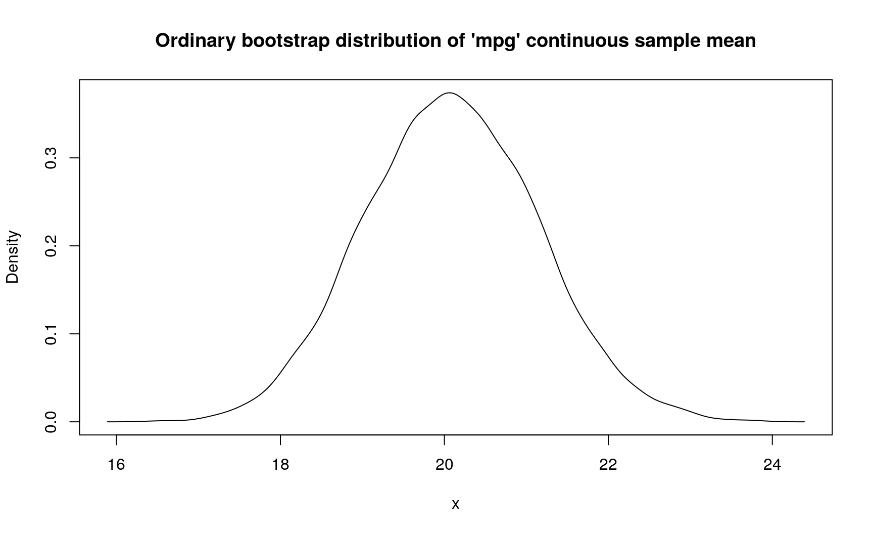
One can also do ordinary bootstrap but represent bootstrap distribution of sample mean with continuous random variable:

# Using ordinary bootstrap, but treating sample mean as continuous
d_mpg_con_mean_2 <- mtcars$mpg %>% 
  new_d(type = "discrete") %>% 
  form_estimate(
    stat = mean, sample_size = nrow(mtcars),
    # Create continuous pdqr-function from bootstrap sample means
    args_new = list(type = "continuous")
  )

summ_sd(d_mpg_con_mean_2)
## [1] 1.063524

plot(
  d_mpg_con_mean_2,
  main = "Ordinary bootstrap distribution of 'mpg' continuous sample mean"
)

In this case, sample mean has standard deviation from 1.04067 to 1.1539572 (depends on assumptions about data generating process).

Example 2: single logical estimate

Share of 4-cylinder cars in mtcars is equal to 0.34375. However, it might happen that we don’t care about actual value, but only if it is bigger 0.3 or not. In present data it is bigger, but how sure we can be about that? In other words: if we repeat sampling sets of 32 cars from general population of all cars, which part of it will have share of 4-cylinder cars bigger than 0.3?. Here is the way of computing that with ‘pdqr’:

# If statistic returns logical value (indicating presence of some feature in
# sample), output estimate pdqr-function is "boolean": "discrete" type function
# with elements being exactly 0 (indicating `FALSE`) and 1 (indicating `TRUE`).
d_cyl_lgl <- mtcars$cyl %>% 
  new_d(type = "discrete") %>% 
  form_estimate(
    stat = function(x) {mean(x == 4) > 0.3},
    sample_size = nrow(mtcars)
  )

d_cyl_lgl
## Probability mass function of discrete type
## Support: [0, 1] (2 elements, probability of 1: 0.7113)

  # To extract certain probability from boolean pdqr-function, use
  # `summ_prob_*()` functions
summ_prob_true(d_cyl_lgl)
## [1] 0.7113
summ_prob_false(d_cyl_lgl)
## [1] 0.2887

In this case, estimated probability that share of 4-cylinder cars in general population is more than 0.3 is 0.7113.

Example 3: comparison of estimates

In mtcars there are 19 cars with automatic transmission (‘am’ variable is 0) and 13 with manual (‘am’ variable is 1). We might be concerned with the following question: are cars with automatic transmission heavier than cars with manual transmission? This is an example of question where reformulating is very crucial, because it leads to completely different methodologies. Basically, it is all about dealing with statistical uncertainty and how to measure that one numerical set is bigger than the other.

First, rather verbose, way of expanding this question is this one: if we randomly choose a car with automatic transmission (uniformly on set of all cars with automatic transmission) and a car with manual (uniformly on set of all cars with manual transmission), what is the probability that weight of the first one is bigger than the second one?. With ‘pdqr’ this can be computed straightforwardly by comparing two random variables (which is implemented exactly like the question above; read more here):

# Seems reasonable to treat weight as continuous random variable. Note that this
# means use of kernel density estimation, which can lead to random variable that
# returns negative values. As weight can be only positive, it is a good idea to
# ensure that. Package 'pdqr' has `form_resupport()` function for that.
d_wt_am0 <- mtcars$wt[mtcars$am == 0] %>%
  new_d(type = "continuous") %>% 
  # Ensure that returned values are only positive
  form_resupport(c(0, NA))
d_wt_am1 <- mtcars$wt[mtcars$am == 1] %>%
  new_d(type = "continuous") %>% 
  form_resupport(c(0, NA))

# Comparing two pdqr-functions with `>=` results into boolean pdqr-function
summ_prob_true(d_wt_am0 >= d_wt_am1)
## [1] 0.9209063

So in this case the answer is that probability of “automatic” cars being heavier than “manual” ones is around 0.921.

Second way of understanding question about comparing is the following: is average weight of “automatic” cars bigger than of “manual”?. This type of questions are more widespread in statistical practice. Having to deal with statistical uncertainty, this should be reformulated: if we repeat sampling (in parallel pairs) sets of 19 “automatic” cars and of 13 “manual” cars, which part of the set pairs will have mean weight of “automatic” cars bigger? This question implies creating bootstrap distribution of sample means for “automatic” and “manual” cars with the following comparing:

d_wt_am0_mean <- d_wt_am0 %>% 
  form_estimate(stat = mean, sample_size = sum(mtcars$am == 0)) %>% 
  # Ensure "positiveness" of random variable
  form_resupport(c(0, NA))
d_wt_am1_mean <- d_wt_am1 %>% 
  form_estimate(stat = mean, sample_size = sum(mtcars$am == 1)) %>% 
  form_resupport(c(0, NA))

# Comparing two random variables representing sample means
summ_prob_true(d_wt_am0_mean >= d_wt_am1_mean)
## [1] 1

So in this case the answer is that probability of “automatic” cars being heavier than “manual” ones is 1.

Computed results can have decisively different outcomes. If researcher sets a standard 0.95 rule, first variant would imply that conclusion ‘“automatic” cars are heavier than “manual”’ isn’t significant, while the second would imply otherwise.